
Standard data products are a bit of a misnomer for DL-NIRSP as the instrument is designed to be very flexible, and thus the characteristics of various datasets can vary widely. Still, DL-NIRSP defines standard configurations and timing modes that lead to standard data products to provide an efficient means for users to understand and design basic DL-NIRSP programs.
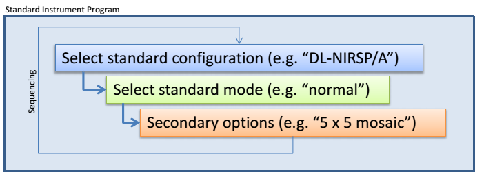
To the potential user, creating an instrument program using standard data sets represents the most straightforward, simple manner in which to design DL-NIRSP observations. For standard observations, the potential user first chooses a standard configuration based on the scientific observables necessary to address the science topic. The user then selects a standard mode based on the need for temporal resolution versus polarimetric sensitivity. Finally, a minimum number of secondary options, such as the number of spatial steps, can be specified either by default or according to the user's needs. Sequences of these standard observations combine to form a DL-NIRSP instrument program.
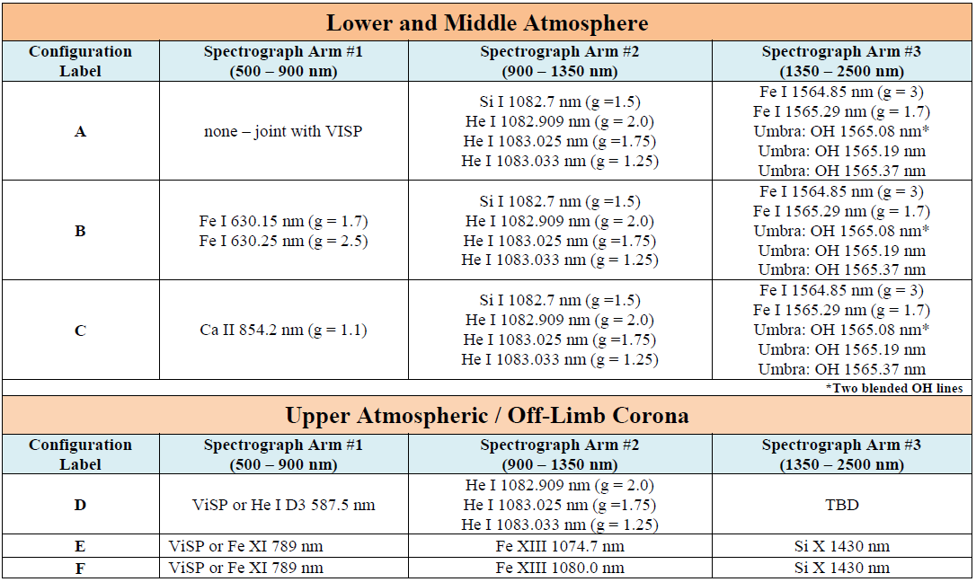
DL-NIRSP can target diverse phenomena throughout the solar atmosphere, viewe both on-disk and off-limb. In general, solar observations with DL-NIRSP can be segmented into two primary categories to allow the definition of the standard observing configurations. The first category targets the lower and middle solar atmosphere on-disk where thermal widths dictate the need for higher spectral resolution. The second category encapsulates much of the upper atmospheric science of the corona viewed off-limb. DL-NIRSP adopts these categories, and further defines the spectral channels for three standard configurations for each category, as shown in Table 1. Standard configurations can be referred to by the instrument name and the configuration letter label. For example, DLNIRSP-A refers to a configuration in which arm #2 targets the He I 1083 nm channel and arm #3 targets the Fe I 1565 nm spectral channel.
Standard data sets are first specified by a DL-NIRSP standard configuration and then by an instrument timing mode, which will specify all instrument exposure timing and coordination information for a given observation. The default polarimeter setting will be 8-state modulation by a continuously rotating modulator in every mode.
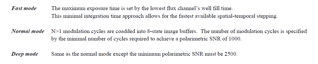
Adopting the familiar terminology of the Hinode-SP standard observing modes, DL-NIRSP will employ three different observing modes for standard observations: Fast, Normal, and Deep. While the specific settings will vary by the configuration, the generalized definitions for each mode are as follows:
Objective:
To probe the small-scale dynamics of solar magnetic structures both in the photosphere and chromosphere so to understand the energetic coupling of the solar atmosphere.
Overview:
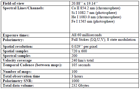
In this use case, DL-NIRSP is configured with the DL-NIRSP standard configuration C in normal timing mode to obtain high spatial resolution observations with a 0.029'' sampling resolution over a 20.88'' x 19.14'' field-of-view, approximately the extent of a rosette concentration of dark chromospheric mottles at network boundaries. The data cube resulting from the observation has 720 spatial x-samples, 660 spatial y-samples, and 200 wavelength samples.
The field-scanning mirror mosaics the field with a 9 x 11 scanning geometry. The spectrograph is operating with a spectral resolution of R ~ 250,000. The polarimeter samples 16 modulation states in one rotation of the continuously rotating polychromatic modulator. The exposure times of the three cameras for each modulation state are set according to the photon flux at each wavelength and the detector presumed full well depth (100,000e-). Exposure times are also balanced to allow proper synchronization. In this case, the well filling of the visible channel was reduced to 80 percent of the full well. For each tile of the 9 x 11 mosaic, one full rotation of the modulator is performed, resulting in a total of 16 individual exposures that are co-added into 8 unique modulation states.
For a single mosaic tile (i.e. a single position of the field scanning mirror), 16 exposures are acquired. These 16 exposures require 960 msec to complete and are subsequently transferred to the data handling system in 8 accumulated buffers. In this case, each individual exposure within the first 8 exposures are coadded by the camera controller to their counterpart in the second set of 8 exposures, resulting in 8 frames worth of outputted data from 16 exposures. Assuming 100 msec for the move of the field-scanning mirror between tiles, a full 9 x 11 mosaic is recorded in a total of 105 seconds. Repeating the mosaic 100 times results in a 3 hour time sequence.
This nominal use case results on average in 7.33 archived detector frames per second per detector.
Derived Physical Parameters (i.e. "Observables")
From the described use case and data set/product, here is a small subset of the physical information and reduced parameters available from an analysis of this data: